Image Warping and Mosaicing (Part A)
In this project I make use of homographies to warp images such that transforms between images are projective. This is a technique often used to create panoramas.
Taking Images
I took two images of the campanile standing in the same spot but slightly turning my phone for the second photo. I also took several photos of rectanuglar objects in my room to rectify as well as some other scenes that I anticipate mosaicing.
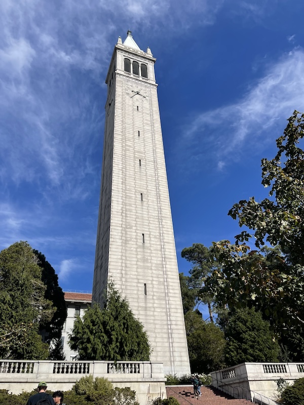
Campanile Image 1
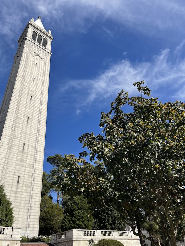
Campanile Image 2
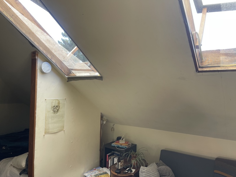
Room Image 1
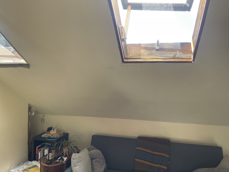
Room Image 2
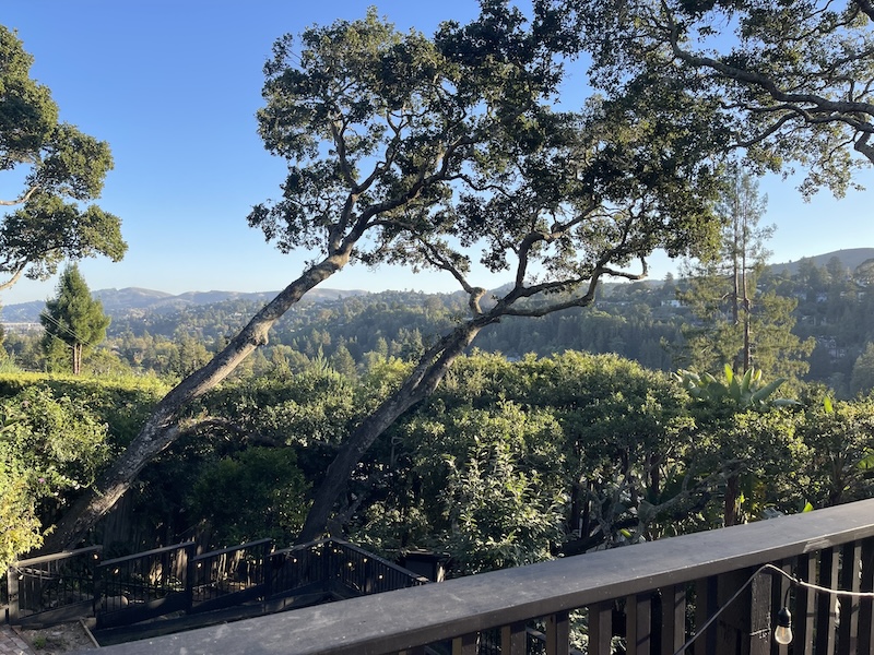
Landscape Image 1
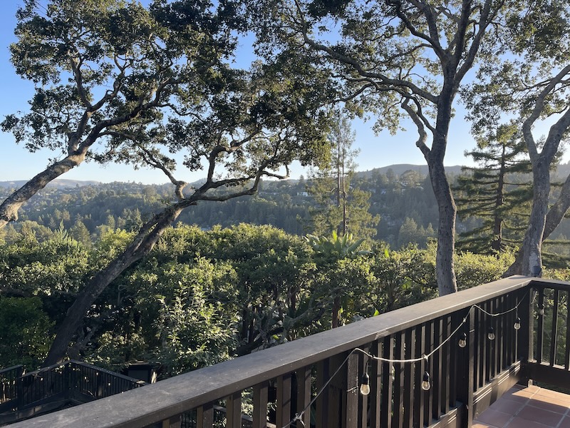
Landscape Image 2
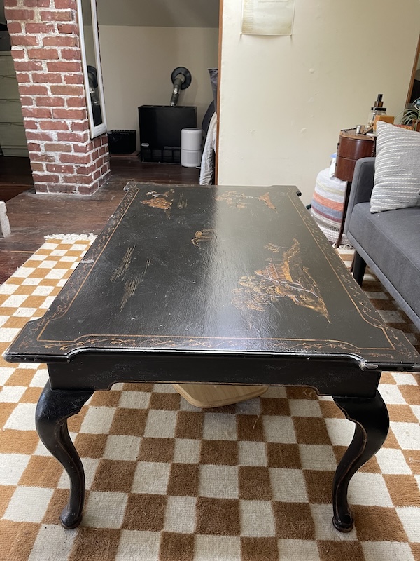
Coffee Table
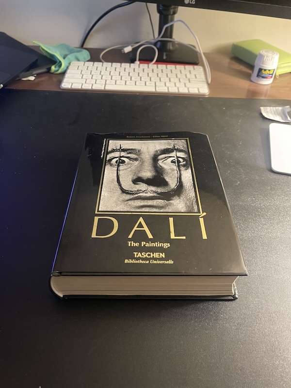
Dali Book
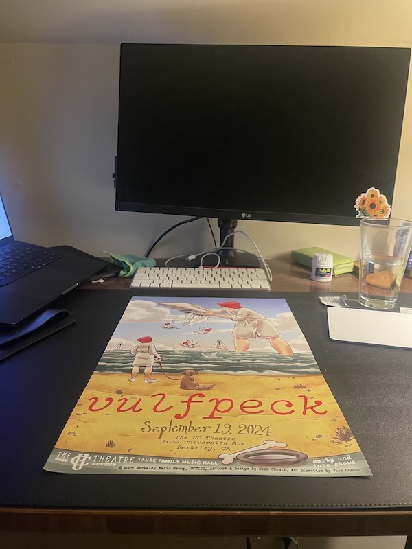
Vulfpeck Poster
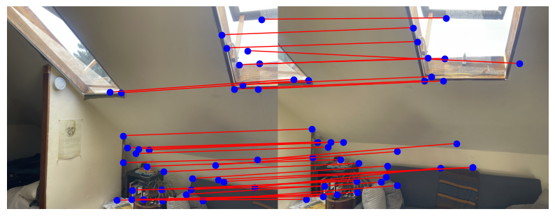
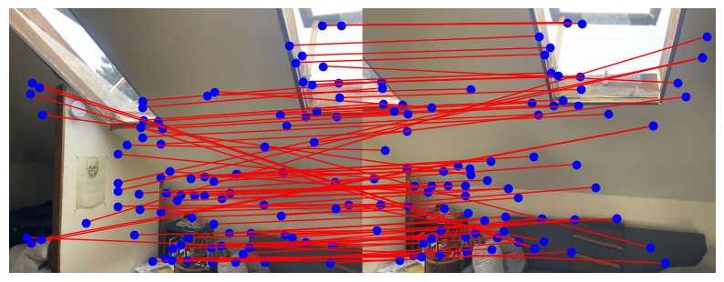
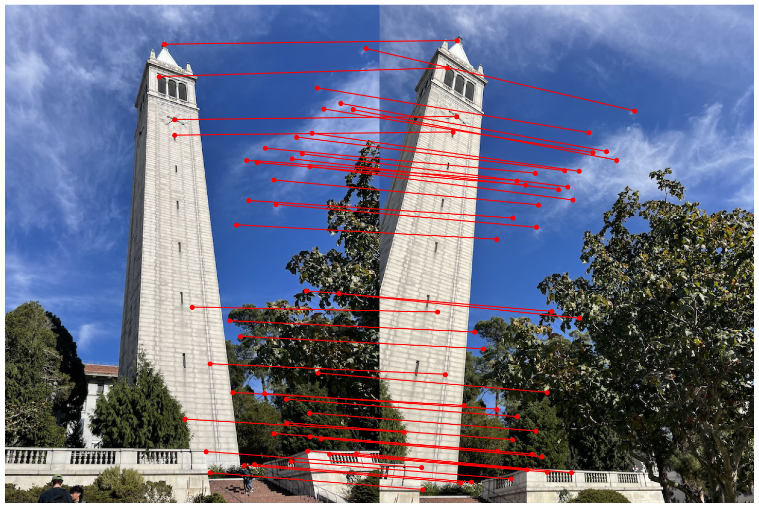
Recovering Homographies
A homography is a transformation that maps points from one plane to another using a 3x3 matrix. Given two images, we want to find the homography matrix H such that corresponding points in both images satisfy:
Here, p and p' are homogeneous coordinates of corresponding points in the two images, and H is the 3x3 homography matrix. To recover H, we need a set of point correspondences between the two images.
Setting up the System of Equations
The homography matrix H has 8 degrees of freedom (since the 9th element can be set to 1 for scaling). Given at least 4 pairs of corresponding points, we can solve for the elements of H using a system of linear equations.
For each pair of points (x, y) in the first image and (x', y') in the second image, we can derive the following equations:
y' = h4*x + h5*y + h6
w' = h7*x + h8*y + 1
To eliminate the non-linear dependency on w', we divide by w' and express the system as:
y' = (h4*x + h5*y + h6) / (h7*x + h8*y + 1)
Rearranging the terms, we obtain two linear equations for each correspondence:
y' * (h7*x + h8*y + 1) = h4*x + h5*y + h6
Matrix Form
We can represent the system of equations in matrix form as Ah = b, where h is a vector containing the 8 unknown elements of the homography matrix, and A and b are constructed from the point correspondences.
For each correspondence, the following two rows are added to A:
[ 0, 0, 0, -x, -y, -1, y'*x, y'*y, y']
We can then solve this overdetermined system using a least-squares method to recover the vector h, which can be reshaped into the 3x3 matrix H:
[h1 h2 h3
h4 h5 h6
h7 h8 1]
Application
Once the homography matrix H is computed, it can be used to warp one image into the coordinate space of another image, or to rectify an image by mapping it to a known geometric shape (e.g., a square or rectangle).
Warping Images
Once the homography is estimated, the next step is to re-project one image onto another to create a seamless stitch. Let's assume we are projecting Image 1 onto Image 2. To ensure smooth re-projection, we use an inverse warp technique. This begins by calculating the bounding box for the final image. We first take the four corners of Image 1 and apply the homography to map it onto the coordinate space of Image 2, determining the area where the final image will appear. Next, we interpolate the pixel values from Image 1 to find their corresponding locations in the output image.
Image Rectification
To confirm that my warping function and homography is working correctly, I rectified a few images. This means taking photos of a rectangualr object at an angle so that the object does not appear perfectly rectangualr, then warping that image onto a rectangle to show the object 'straight on'

Coffee Table
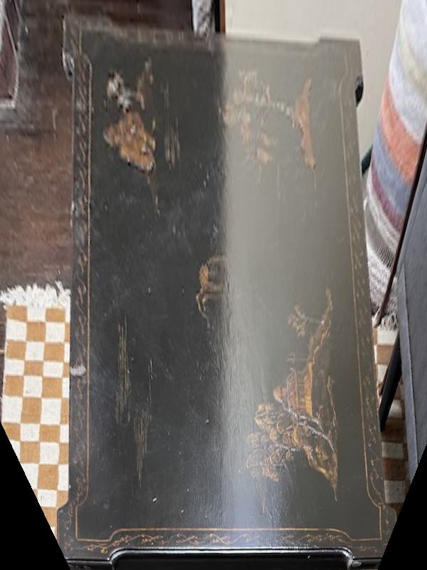
Rectified Coffee Table Rectified

Dali Book
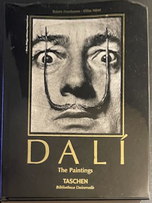
Rectified Dali Book

Vulfpeck Poster
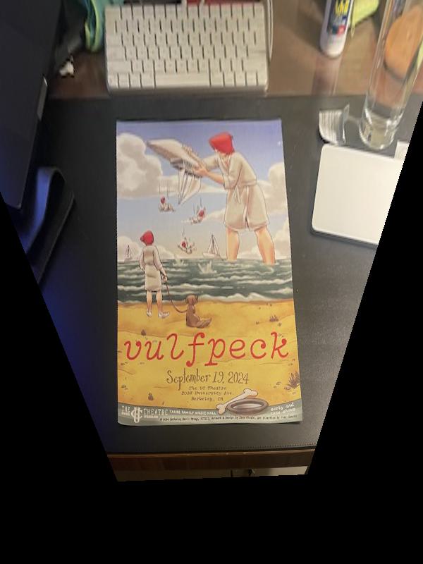
Rectified Vulfpeck Poster
Blend the images into a mosaic
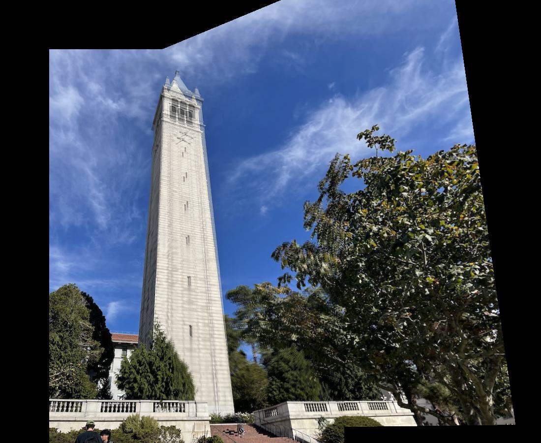
Now for the fun part I blended together images to create a mosaic. I used my two images of the campanile. The means to do this is to use my warp function to warp one image onto the other using the homography created from the correspondence points. Next you need to stitch the images together. However, if you simply just take an average of pixels when stitching them together you will get inconsistent results. A better option is to use blending with an alpha mask which allows for a smooth transition where the imags overlap. You further need to keep track of if a given pixel is contributed to by one or two images and normalize accordingly.

Image 1

Image 2
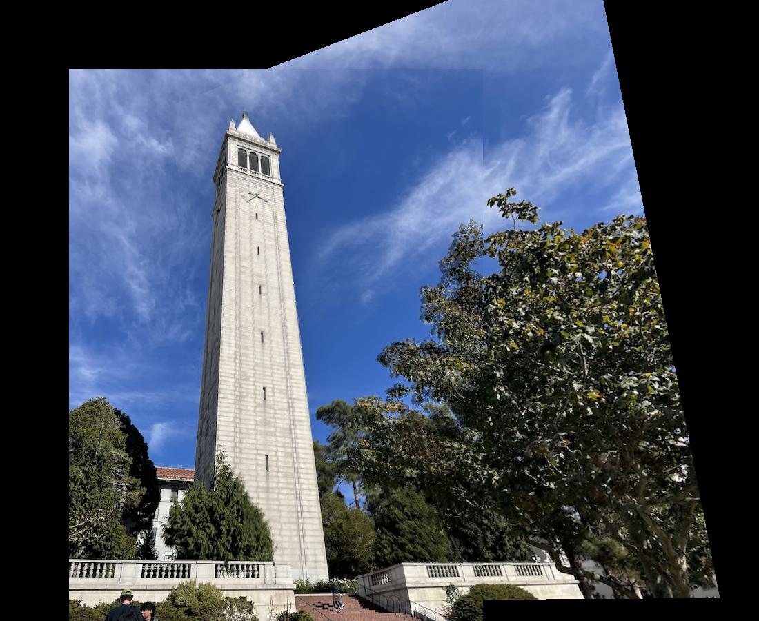
Mosaiced Campanile
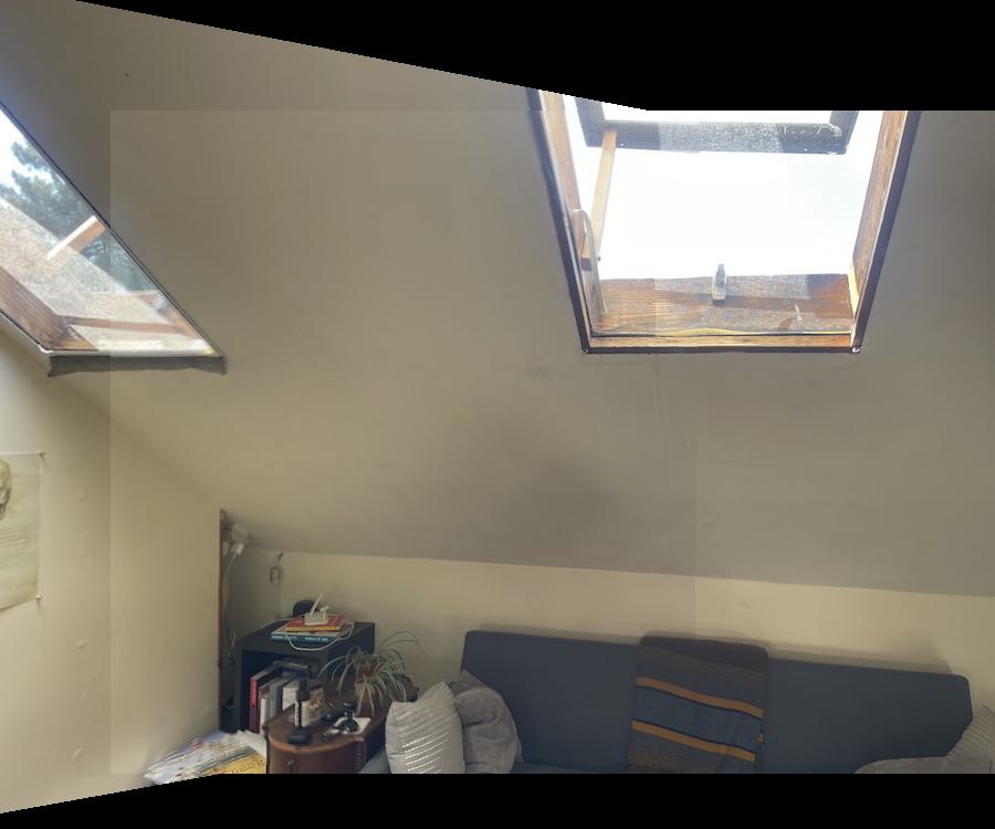
You might notice in the bottom middle of my image there is an edge where the images don't line up too well. This is due to the fact that I turned my body instead of the camera when taking these photos. This inspired me to take more photos of the inside of my room and a beautiful landscape to create more mosaics, this time being careful to only turn the camera around its focal point. Below are the results of these mosaics.

Image 1

Image 2
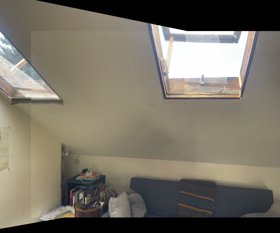
Mosaiced Room

Image 1

Image 2
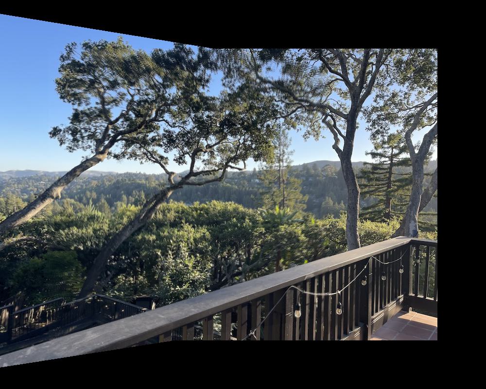
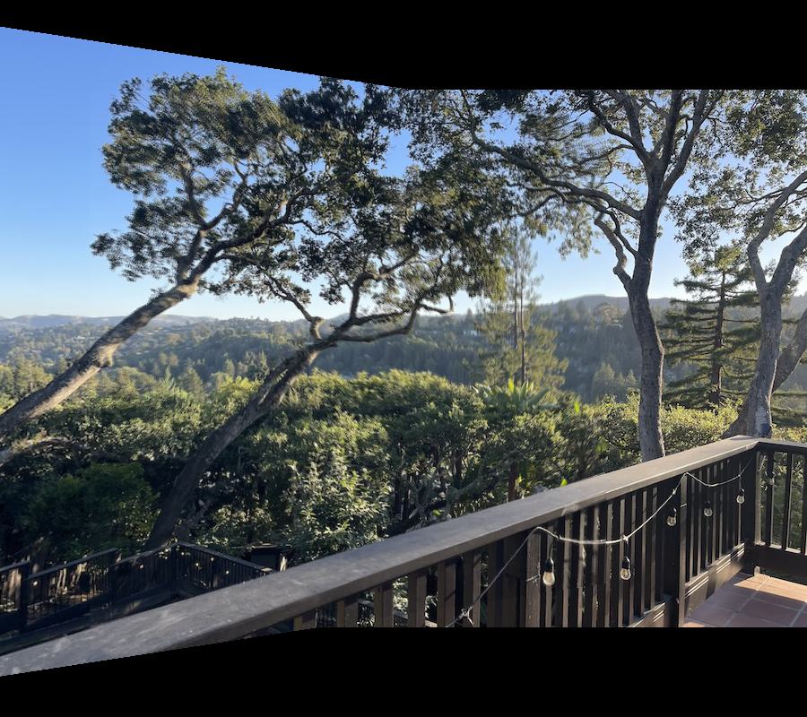
Mosaiced Landscape
