The Power of Diffusion Models! (Part A)
In this project I implement diffusion loops and leverage them for various image generation tasks like inpainting and creating visual anagrams or hybrid images.
Part 0: A few examples with DeepFloyd
"DeepFloyd" is a two stage Diffusion model trained by Stability AI. The first stage generates 64 x 64 images and then upsamples them 256 x 256. Below are some outputs with varrying numbers of iteratives steps which dictate how many denoising steps are taken. As supported by the images, as you take more steps you get clearer more detailed imagse but the runtime increases quite a bit, consequently.
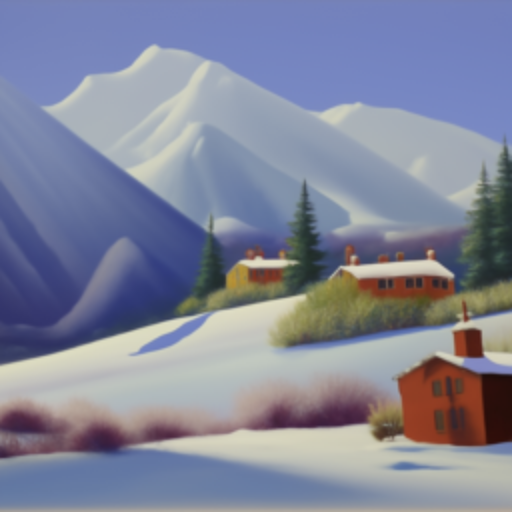
"an oil painting of a snowy mountain village" 10 iteratitions 256x256
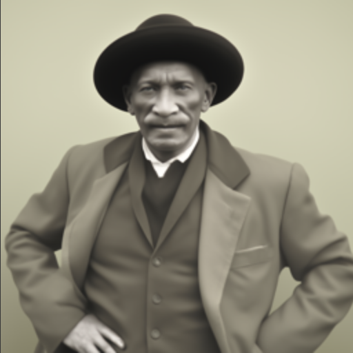
"a man wearing a hat" 10 iterations 256x256
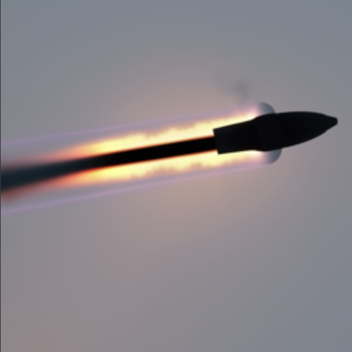
"a rocket ship" 10 iterations 256x256
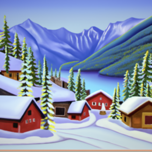
"an oil painting of a snowy mountain village" 20 iteratitions 256x256
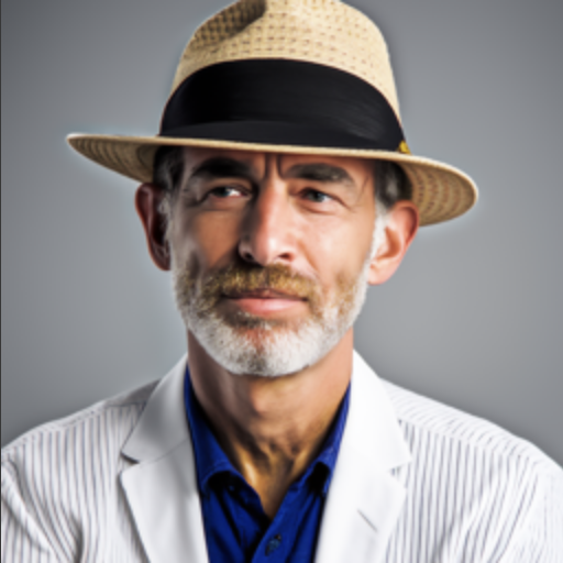
"a man wearing a hat" 20 iterations 256x256
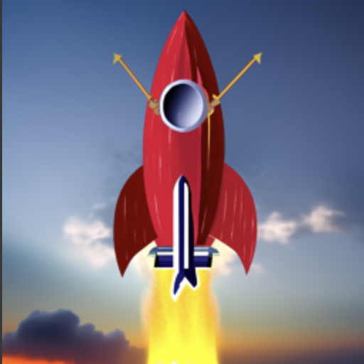
"a rocket ship" 20 iterations 256x256
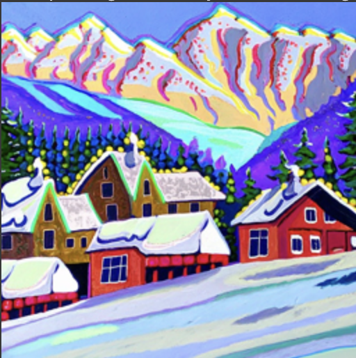
"an oil painting of a snowy mountain village" 500 iteratitions 256x256
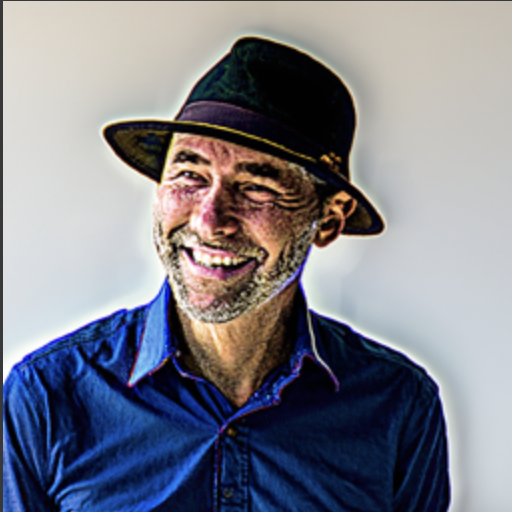
"a man wearing a hat" 500 iterations 256x256
"a rocket ship" 500 iterations 256x256
Part 1.1 Forward Pass of sampling loop.
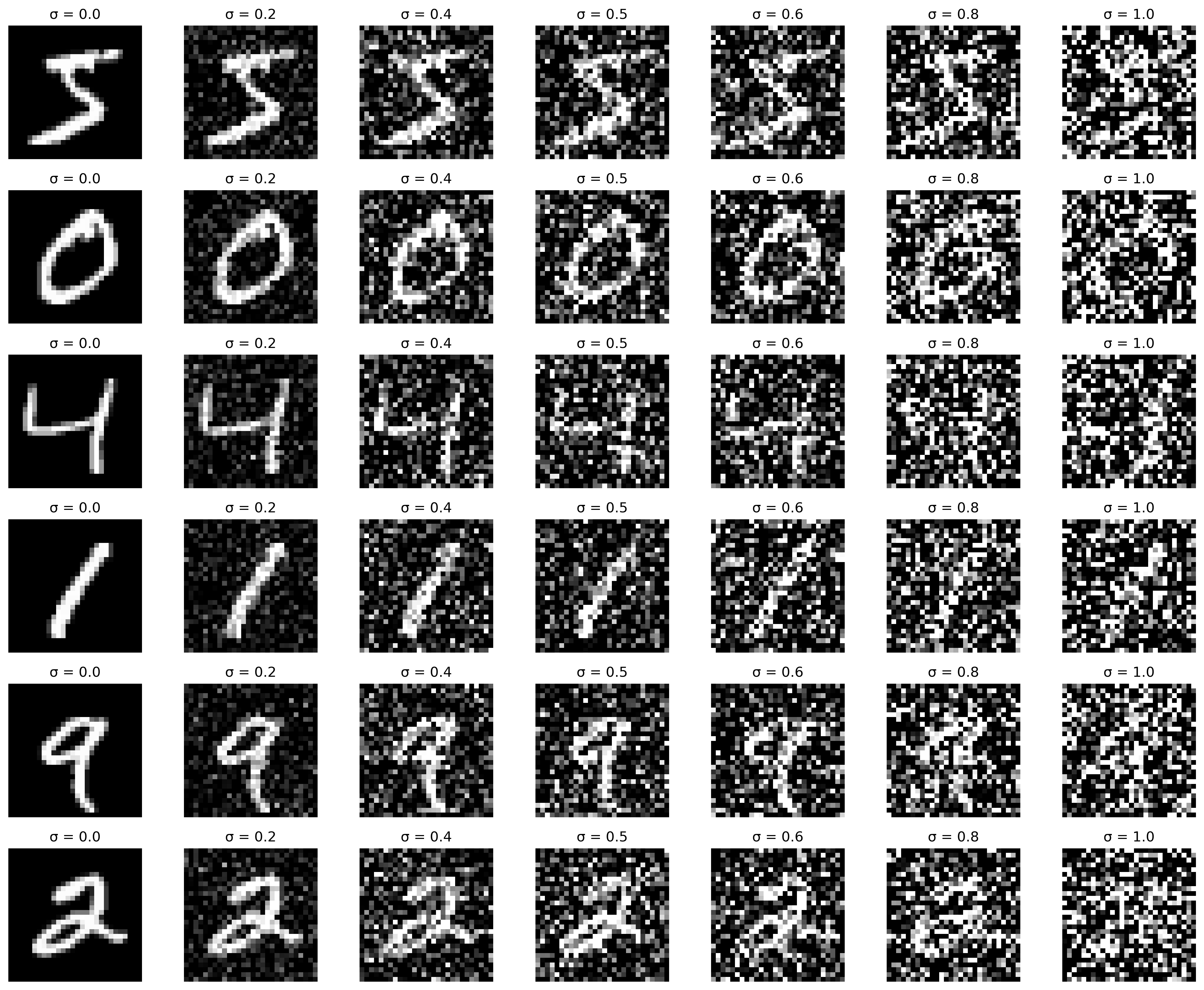
The idea of a sampling loop is to begin with a clean image x0 and progressively add more noise to this image giving xt until at timestep t=T we have in image of essentially pure noise. The goal of a diffusion model is to remove this noise by predicting the noise in an image.
The first step is the forward pass, which encompasses adding noise to a clean image. This process is defined by the formula:
xt = √αt x0 + √1 - αt ε
where αt is the noise coefficient. Below are noisy images at various t values for a sample image of the campanile.
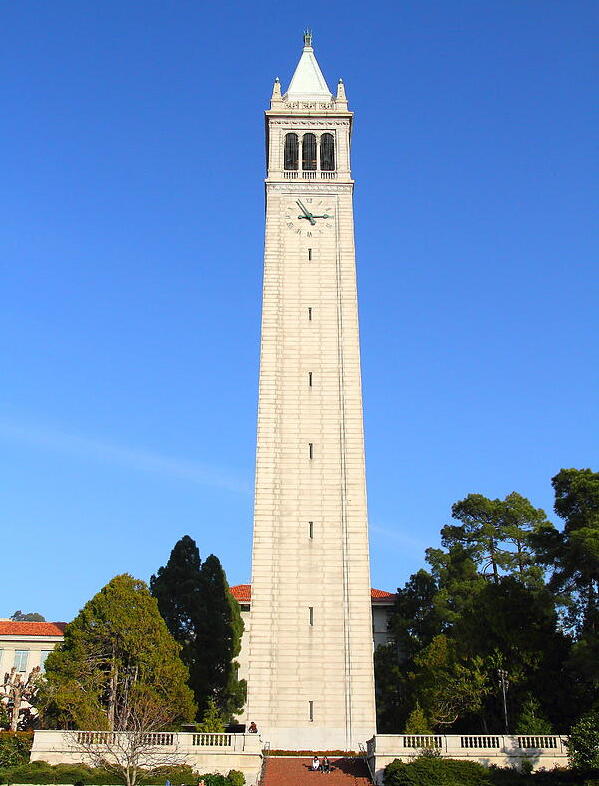
Berkeley Campanile

Campanile at t = 250

Campanile at t = 500

Campanile at t = 750
Part 1.2 Classical Denoising
A basic approach to denoising is to use a Gaussian blurr to remove the noise in the image, however as seen below the results are not so great.
Campanile at t = 250
Campanile at t = 500
Campanile at t = 750

Campanile at t = 250 Denoised

Campanile at t = 500 Denoised

Campanile at t = 750 Denoised
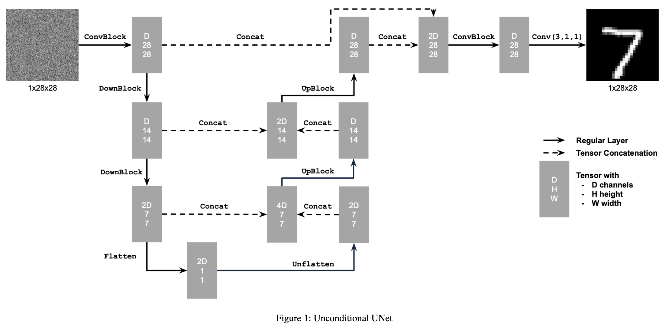
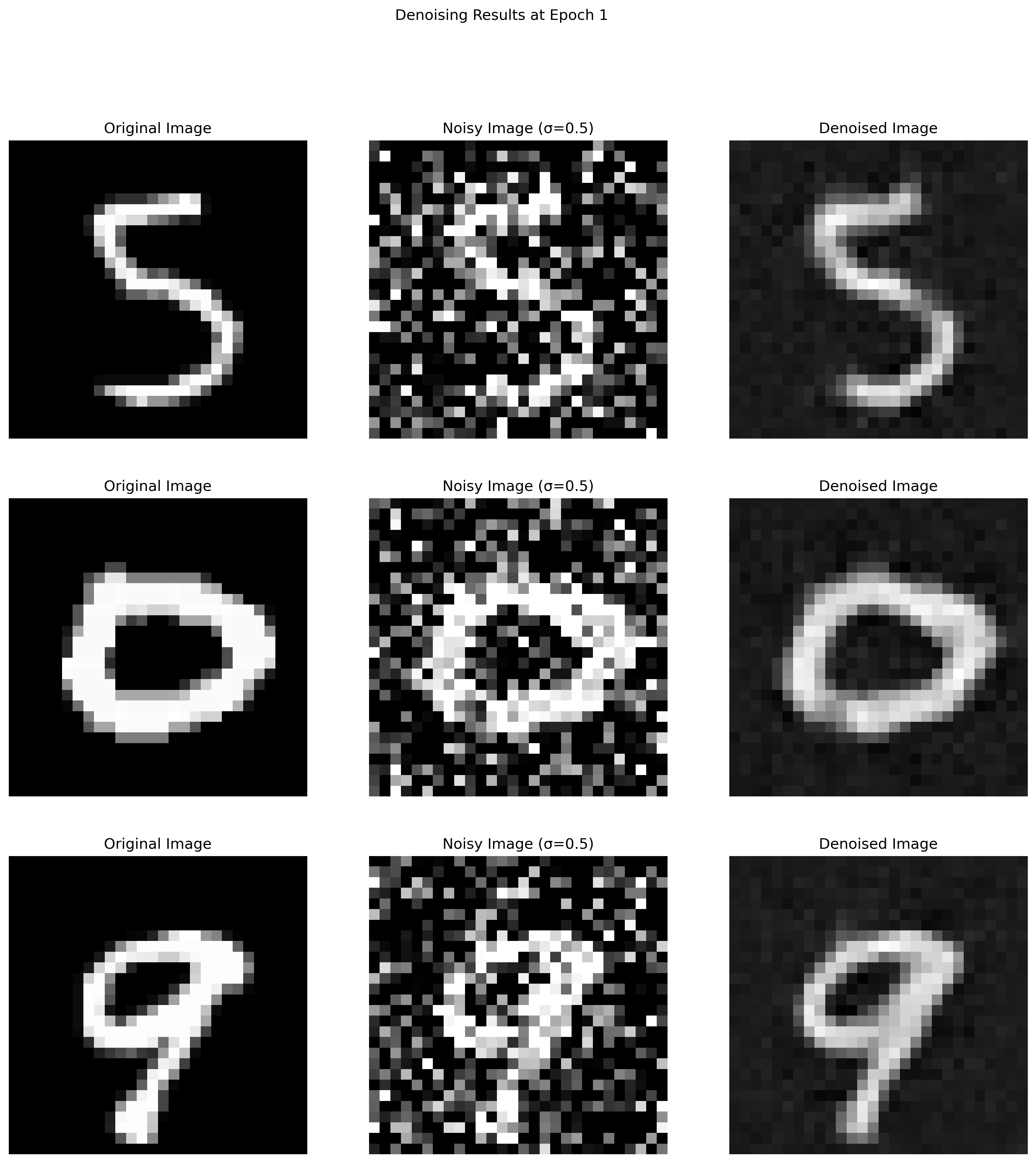
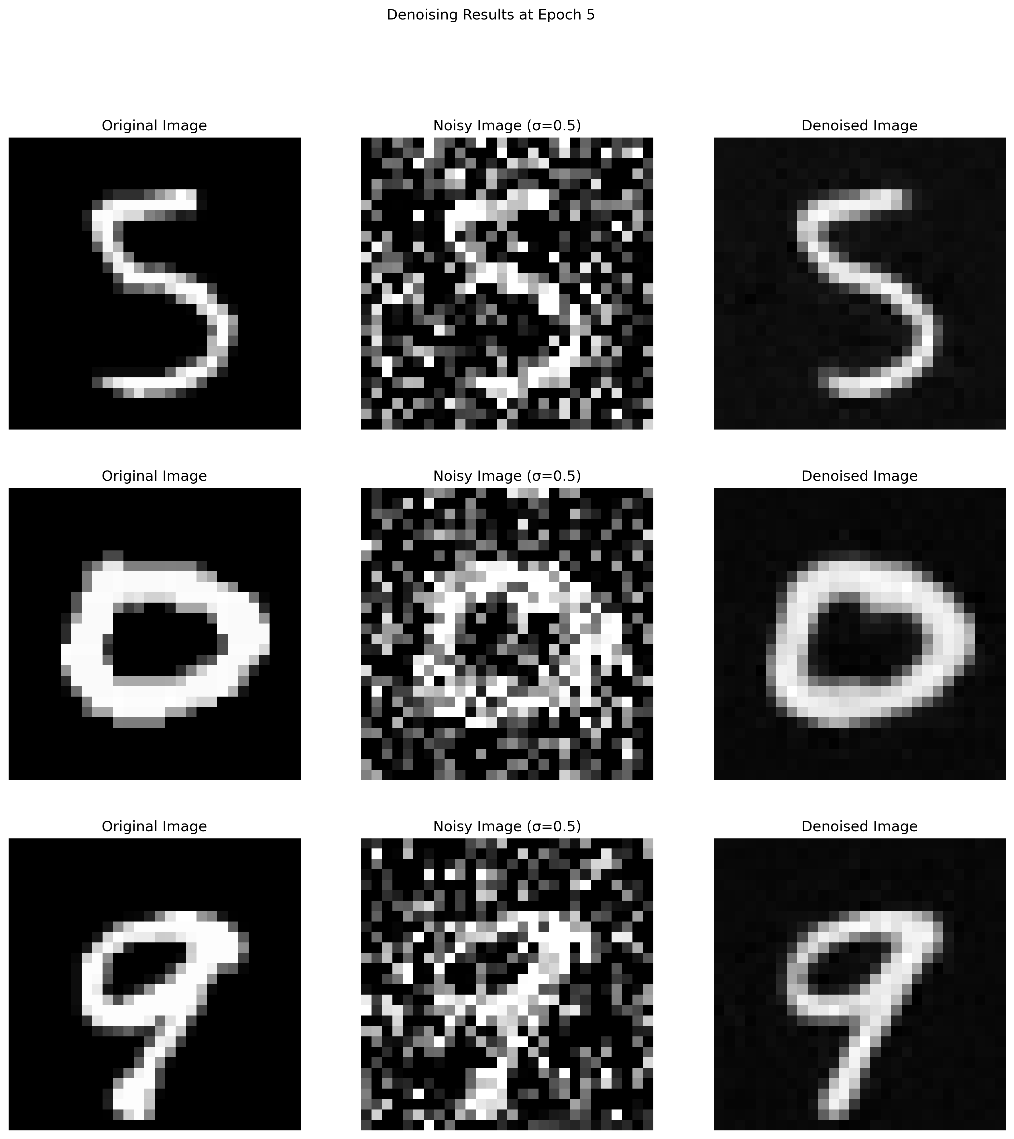
Part 1.3 One-Step Denoising
For this part we use a pretrained UNet to recover gaussian noise dorm the image and then remove this noise and in theory getr something close to the original image. I ran this for t = [250, 500, 750] and displayed the images below.

Noisy Campanile at t=250

Noisy Campanile at t=500

Noisy Campanile at t=750

One-Step Denoised Campanile at t=250

One-Step Denoised Campanile at t=500

One-Step Denoised Campanile at t=750
Part 1.4 Iterative Denoising
In the last part we can see that the UNet struggles as you add more noise. For this part we iteratively denoise meaning that we denoise from x1000 to x0 step by step, we do so in strides of 30 to speed this up. The formula for computing the next step is:
\( x_{t'} = \frac{\sqrt{\overline{\alpha_{t'}} \beta_t}}{1 - \overline{\alpha_t}} x_0 + \sqrt{\alpha_t \frac{(1 - \overline{\alpha_{t'}})}{1 - \overline{\alpha_t}}} x_t + v \sigma \)
Where αt = αt ∕ αt'

Noisy Campanile at t=90

Noisy Campanile at t=240

Noisy Campanile at t=390

Noisy Campanile at t=540

Noisy Campanile at t=690
Originial Campanile

Iteratively Denoised Campanile

One-step Denoised Campanile

Gaussian Blurred Campanile
Part 1.5 Diffusion Model Sampling
We can use our iterative denoising to generate images form scratch, passing random noise in and making the text prompt "a high quality photo". Here's 5 results of that below.

Sample 1

Sample 2

Sample 3

Sample 4

Sample 5
Part 1.6 Classifier-Free Guidance (CFG)
The images from the previous section lack in quality and sometimes even appear nonsensical. To improve the results we'll use classifier-free guidance to refine the images by computing two different noise estimates: a conditional noise estimate and an unconditional noise estimate. By combining these two estimates, we can control the balance between diversity and quality in the images we generate.
In CFG, we denote the conditional noise estimate as \( \epsilon_{\text{cond}} \) and the unconditional noise estimate as \( \epsilon_{\text{uncond}} \). Our new noise estimate \( \epsilon \) is then given by:
\[ \epsilon = \epsilon_{\text{uncond}} + s \cdot (\epsilon_{\text{cond}} - \epsilon_{\text{uncond}}) \]
Here, \( s \) is a scaling factor that controls the strength of the guidance. By adjusting \( s \), we can achieve different effects:
- When \( s = 0 \), we obtain a purely unconditional noise estimate.
- When \( s = 1 \), we recover the conditional noise estimate.
- For values \( s > 1 \), we achieve enhanced image quality, often at the expense of diversity.
The true "magic" of CFG happens when \( s > 1 \). In this case, the generated images are often much higher in quality, providing clearer and more meaningful visuals compared to the unguided generation process.

Sample 1 with CFG

Sample 2 with CFG

Sample 3 with CFG

Sample 4 with CFG

Sample 5 with CFG
Part 1.7 Image-to-image Translation
We can take what we did in 1.4 and by adding more noise we force our algorithm to make a larger edit in hopes that it will be "creative" i.e. hallucinate a bit and produce something cool. This can be thought of as forcing a noisy image back onto the manifold of natural images. I tried this with varrying values for the starting index, and you can see that as the edits go on the image looks more like the original.

i_start = 1

i_start = 3

i_start = 5

i_start = 7

i_start = 10

i_start = 20
Part 1.7.1 Editing Hand-Drawn and Web Images
The procedure above works even better if you start with a nonrealistic image like a drawing or painting and project it onto the manifold of natural images. I've done this with some images from the web as well as a few hand drawn scribbles.

Avocado i_start = 1

Avocado i_start = 3

Avocado i_start = 5

Avocado i_start = 7
Avocado i_start = 10

Avocado i_start = 20

Avocado original

Apple scribble i_start = 1

Apple scribble i_start = 3

Apple scribble i_start = 5

Apple scribble i_start = 7

Apple scribble i_start = 10

Apple scribble i_start = 20

Apple scribble original

Man scribble i_start = 1

Man scribble i_start = 3

Man scribble i_start = 5

Man scribble i_start = 7

Man scribble i_start = 10

Man scribble i_start = 20

Man original
Part 1.7.2 Inpainting
We can use a mask to create an image that has the original content of the image in some parts, but generated content in other parts. For this I put a mask over the upper portion of the campanile and generated a few results.
.png)
Sample 1
.png)
Sample 2
.png)
Sample 3
.png)
Sample 4
.png)
Sample 5

Sample 1

Sample 2

Sample 3

Sample 4

Sample 5
Original

Mask

Sample 1

Sample 2

Sample 3

Sample 4

Sample 5
Original

Mask
Part 1.7.3 Text-Conditional Image-to-image Translation
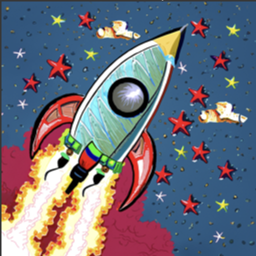
We can add control to our previous results by changing th etext promp from "a high quality photo" to something more descriptive like "a rocket ship". The results below are for increasing values of i_start, as i_Start increases the model gets less "creative" and the output looks more like the input image.

Rocket ship at i_start=1

Rocket ship at i_start=3

Rocket ship at i_start=5

Rocket ship at i_start=7

Rocket ship at i_start=10

Rocket ship at i_start=20

Pencil at i_start=1

Pencil at i_start=3

Pencil at i_start=5

Pencil at i_start=7

Pencil at i_start=10

Pencil at i_start=20

Waterfall at i_start=1

Waterfall at i_start=3

Waterfall at i_start=5

Waterfall at i_start=7

Waterfall at i_start=10

Waterfall at i_start=20
Part 1.8 Visual Anagrams
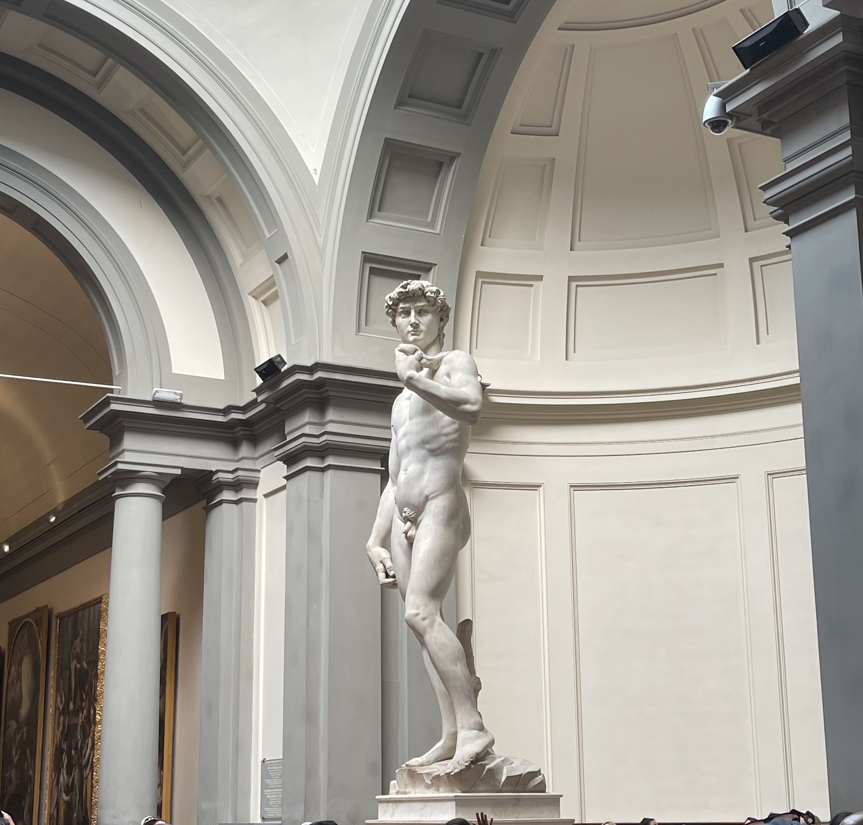
Getting even more creative we can create an image that looks like one thing right side up and another thing upside down, similar to Salvador Dali's Elephants Reflecting Swans. The idea is to compute two noises, one for a given prompt for example "an oil painting of an old man" and another for the same image but flipped and with the prompt "an oil painting of people around a campfire". Then, average these two noises and use that as your noise.
.jpg)
"Oil painting of an old man"

"A photo of a man""

"An oil painting of a snowy mountain village"

"a photo of the amalfi cost"
"An oil painting of people around a campfire"
"A photo of a dog"
"A lithograph of a waterfall"
"A lithograph of a skull"
Part 1.9 Hybrid Images
Similar to project 2 where I took advantage of the way humans percieve high and low frequnecy visual data, we can use a diffusion model to mkae factorized images that look like one thing from a far and another from close up. The idea is similar to the previous par tbut instead of flipping the image we just run a high pass and low pass filter on the image and take the noise with respect to two different text prompts, then sum this noise to get our overall noise. The results from this part are not as pleasing as the Visual Anagrams, I palyed around with tryong to weight the noise differently with emphasis on the "harder" prompt but still many of my images look dissatisfying.

"A lithograph of a skull" and "A lithograph of a waterfall"

"An oil painting of a snowy mountain village" and "A lithograph of a waterfall"

"A lithograph of a skull" and "a photo of the amalfi cost"
.jpg)
"A lithograph of a skull" and "a photo of the amalfi cost" w/ emphasis on amalfi.
Conclusion
This project was quite challenging and involved lots of trial and error with different input images and prompts and playing around with how to use the noise appropriately. However, it was quite rewarding and provided great insight into the capabilities of diffusion models and how to get creative and create some fun images that mess with human perception.

.png)