Augmented Reality Project Overview
In this project I insert a synthetic object into a video I captured which is a basic fundamental of AR. The idea is to use 2D points from the video and 3D coordinates that are known to calibrate the camera for each frame and use projection matrix to project the 3D coordinates of your synthetic object into your 2D frames in the video.
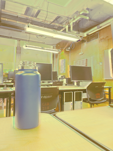
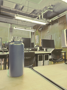
Input Video
I drew a regular grid pattern on a box so that I could easily annotate the points and measure their real 3D coordinates. I then took a simply video in which I pan around the box.
Input Video
Keypoints with known 3D world coordinates
The first step is to extract the first frame from the video and annotate some keypoints for that image, I chose to annotate 32 keypoints in the end.
Next, you need to define 3D cooridinates for those same points. Since I drew a grid with 2 inch spacing on my box, I was easily able to define 3D coordinates for each of my 2D keypoints.
Now that we have 2D keypoints for the first frame we need to propogate those for each frame in the video.
To do this I used cv2.calcOpticalFlowPyrLK which is Optical Flow with the Lucas-Kanade method for feature point tracking. It computes the motion of a list of points between two frames by using local gradients of pixel intensities to get the displacement. There were some points that it struggled to properly track which gave weird results, so I simply removed those points from my projection matrix calculation.
Tracking all points
Tracking removed bad points
Calibrating the Camera
Now that we have the 2D points for each frame in the video, we can calibrate the camera by finding a projection matrix that maps the 3D coordinates of points in the world to their corresponding 2D image coordinates. The process involves solving for the camera's projection matrix using the least squares method, which minimizes the error between the predicted and actual 2D points.
To do this, we need to solve the equation:
p = P * X
where p is the 2D point in homogeneous coordinates (x, y, 1), P is the 3x4 camera projection matrix, and X is the 3D point in homogeneous coordinates (X, Y, Z, 1). The goal is to find P that best maps the 3D points to the corresponding 2D points across all frames.
The matrix equation can be rewritten for multiple points as:
[p₁] [x₁ y₁ z₁ 1]
[p₂] [x₂ y₂ z₂ 1]
[p₃] [x₃ y₃ z₃ 1]
... ... ... ...
[pₖ] [xₖ yₖ zₖ 1]
We can solve this system of equations using a least squares approach, where we minimize the sum of squared differences between the actual and predicted 2D points. The resulting matrix P consists of the intrinsic and extrinsic parameters of the camera, which include the camera's focal length, principal point, and orientation in space.
Projecting a cube in the Scene
Now that we have a projection matrix for each frame, we just use it to project the 3D coordinates of our cube onto that 2D frame and then draw the cube onto the frame.
Output Video with Cube
High Dynamic Range Imaging Project Overview
Modern cameras often struggle to capture the full dynamic range of real-world scenes, resulting in images that may be partially underexposed or overexposed. To address this, both photographers and researchers commonly merge data from multiple exposures of the same scene. In this project, you will develop software that automatically combines these multiple exposures into a single high dynamic range (HDR) radiance map and applies tone mapping to convert this map into a displayable image.
This project is based on the Debevec and Malik 1997 paper.
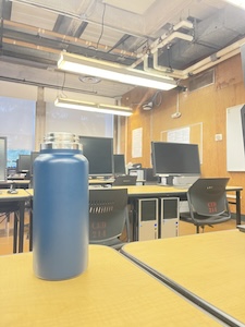
Input Images
We start with images taken at various exposures of a stationary scene, an example shown below.
1/25 sec
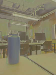
1/4 sec
3 sec
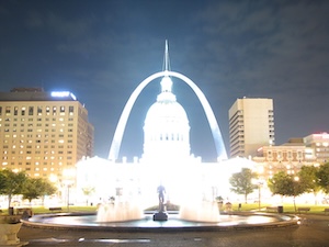
17 sec
Radiance Map Construction
The observed pixel value, Zij, for pixel i in image j is a function of the unknown scene radiance and the known exposure duration:
Zij = f(Ei Δtj). Here, Ei represents the unknown scene radiance at pixel i, and
Ei Δtj denotes the exposure at that pixel. The function f represents the camera's pixel response curve, which is often non-linear.
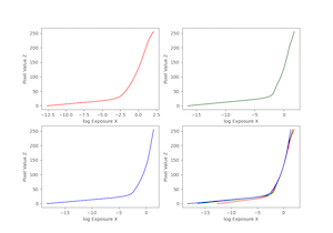
Instead of solving directly for f, we solve for g = ln(f-1), which maps pixel values (0–255) to the logarithm of exposure values. The relationship can be expressed as:
g(Zij) = ln(Ei) + ln(Δtj) (Equation 2, Debevec). Since the scene is static, while we may not know the absolute radiance value Ei, it remains constant across all exposures of the same pixel.
To make the results more robust:
-
Ensure smoothness: A penalty is added to the linear system for large second derivatives of g. The second derivative is approximated as
g(x-1) + g(x+1) - 2g(x), applied across all pixel values except at the boundaries (g(0) and g(255)).
-
Use pixel weighting: Each exposure contributes reliable information only for well-exposed pixels. Weighting is applied according to
Equation 6 in Debevec, using a triangle function that peaks at Z = 127.5 and is zero at Z = 0 and Z = 255.
Once g is solved, radiance values can be calculated using: ln(Ei) = g(Zij) - ln(Δtj) (Equation 5, Debevec).
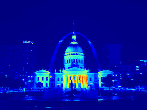
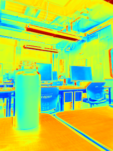
Mean radiance map
Per channel radiance map
Tone Mapping
Once the radiance map is generated, tone mapping is used to compress its dynamic range for display.
We implemented both global and local tone mapping techniques:
Global Tone Mapping
The global method applies a simple compression formula:
E_display = E_world / (1 + E_world). This effectively reduces high-intensity values
while maintaining overall contrast. The result is normalized to the [0, 1] range for display.
Local Tone Mapping
For a more sophisticated approach, we implemented a simplified version of Durand 2002:
- Compute intensity as the average of the RGB channels.
- Extract chrominance as
R/I, G/I, B/I.
- Transform intensity to log space and filter it using a bilateral filter to obtain a base layer.
- Calculate a detail layer as the difference between the log intensity and the base layer.
- Apply scaling and offset to the base layer to control dynamic range compression.
- Reconstruct the intensity by combining the scaled base and detail layers.
- Restore the color by multiplying the intensity with the chrominance and apply gamma compression for display.
The combination of these methods allows for effective visualization of high dynamic range images
while preserving local details and contrast.
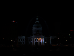
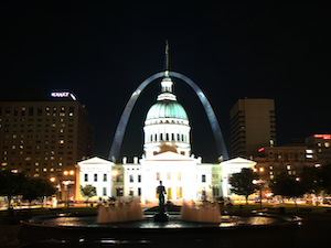
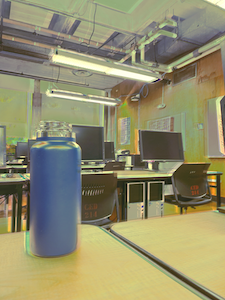
Global Scaling
Global Simple
Durand
Although the difference between the three tone mapping algorithms is not super strong, you can see that the simple scale fails to reduce contrast and some details are lost in the dark. The global simple method is an improvement but it still has some saturation in the darkest and lightest parts of the image. The Durand however remedies this and overall looks quite good.
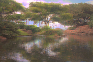
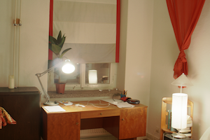
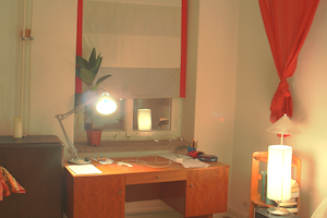
All HDR Images
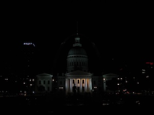
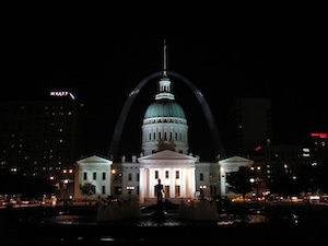
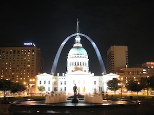
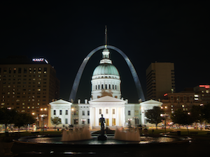
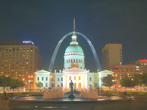
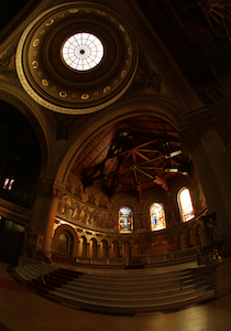
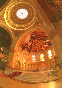
Below are the results for the arch, house, chapel, garage, garden, window, mug, and bonsai for both global simple and Durand tone mapping.
Global Simple
Durand
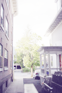
Global Simple
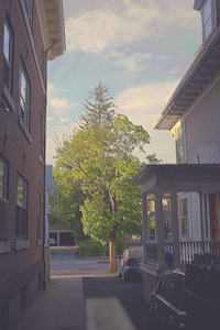
Durand
Global Simple
Durand

Global Simple
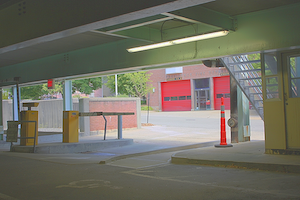
Durand
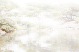
Global Simple
Durand
Global Simple
Durand

Global Simple

Durand
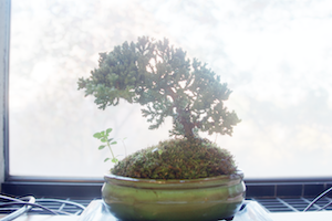
Global Simple
Durand
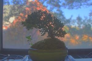
Bells and Whistles!
For Bells and whistles I chose to try HDR on my own images using my iphone camera. I don't have a tripod so I setup some books to hold my phone in place while leaving room for me to adjust the exposure between shots. Unfortunately even the tiny movements from adjusting the exposure and tapping to take the photo messed up the alignment a noticeable amount between images. Nonetheless you can see how the HDR worked below.
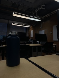
Input 1/120 sec
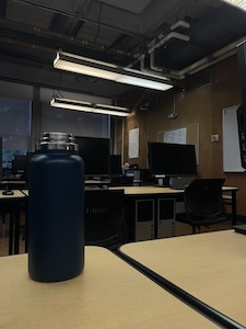
Input 1/60 sec
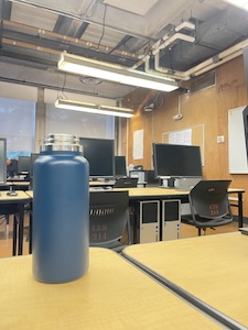
Input 1/40 sec
Input 1/30 sec
Radiance map mean
Radiance map per channel
Global Scale
Global Simple
Durand
Conclusion
This project was quite visually appealing to see my results get better as I debugged. A main challenge in this project was reconstructing the hdr map which took my three implementations before getting solid results. Overall I really enjoyed seeing the results of this project and reading the Debevec paper.